Originally developed in the 1970s and 1980s to tackle control challenges in refineries, Model Predictive Control (MPC) has since become a highly effective advanced control technique widely adopted across numerous industries. When integrated with an optimizer as a multivariable controller, MPC can yield significant advantages.

MPC’s most substantial benefits come to light in applications featuring dead time dominance, constraints, interactions, and a requirement for optimization. It considers the effect of past actions of manipulated and disturbance variables on controlled and constraint variables’ future profile and computes a sequence of controller moves to achieve the desired profile.

Although most MPC applications assume linear process models and use linear programming (LP) for optimization, techniques now exist to incorporate nonlinear modeling and optimization.

MPC finds its most widespread use in the refining and petrochemical industries. It is also employed in other industries such as food processing, pulp and paper, automotive, chemicals, metallurgy, cement, and pharmaceuticals.

This section offers an overview of MPC’s theoretical background and operational fundamentals. It also covers the necessary steps required for MPC implementation, including process analysis and configuration, model development and process testing, MPC simulation, and commissioning.

Model Predictive Control Principles

MPC can be compared to a traditional feedback control loop, but with some important differences. In a feedback loop, the controller receives the error between the set point and the current value of the controlled variable as input. In MPC, the controller uses the error between the predicted future trajectory of the set point and the predicted future trajectory of the controlled variable as input. This error is expressed as a vector of error values over a defined time period in the future.

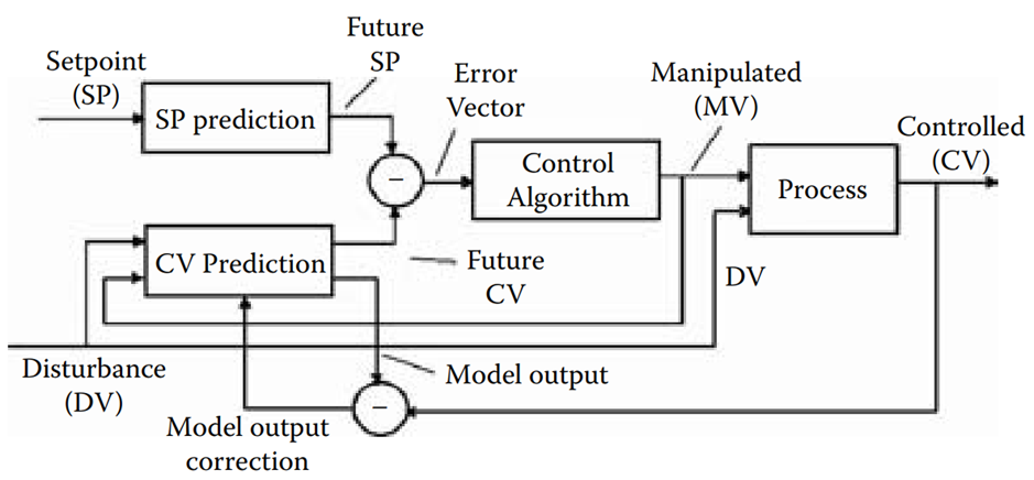
Figure 1.1 [Model predictive control operation diagram. (Copyright 2002, ISA—The Instrumentation, Systems, and Automation Society. All rights reserved. Used with permission of ISA—The Instrumentation, Systems, and Automation Society.)].

Figure 1.1 illustrates an MPC controller for a process with two inputs and one output, and shows how it is similar to a traditional feedback control loop. The controller consists of three components: a process model that predicts the future output of the process, a future trajectory of the set point, and a control algorithm that computes a control action based on the error vector between the two trajectories.

The MPC controller output is a manipulated variable (MV) that is applied to the process input and the process model. A disturbance variable (DV) is also applied as a measured load upset to the process input. The process model predicts the future trajectory of the controlled variable (CV), and any mismatch between the predicted and actual value of the CV is corrected. The predicted CV trajectory is subtracted from the future trajectory of the set point to generate the error vector, which is used as input for the predictive control algorithm. The algorithm calculates outputs to minimize the sum of squared errors over the prediction horizon, taking into account multiple future MV moves.

MPC vs Feedback Control Summary

The differences between an MPC controller and a feedback controller can be summarized as follows:

An MPC controller takes a predicted error vector as input, while a feedback controller uses scalar values of recent errors.
The error vector in an MPC controller is computed by subtracting the corrected model prediction from the future set-point values, while in a feedback controller, the error is the measurement subtracted from the setpoint value.
The MPC controller computes control increments spread over several moves into the future, while only the first move is implemented, and the computation procedure is repeated for the next scan.
An MPC controller considers disturbances with the proper dynamics based on identified models from process step responses in predicting the process output.

To achieve superior performance for processes with long dead times, inverse responses, and higher order dynamics that are challenging to control with a classical PID feedback controller, an accurate process model is critical for the MPC controller’s operation.

MPC controllers are also suitable for multivariable processes as they account for process interactions, handle constraints on the process output and manipulated variables, and integrate and manage optimization. These capabilities make MPC the ideal choice for incorporating process knowledge and solving complex control and optimization problems on the unit operation control level.

Process Modelling

Figure 1.2 illustrates a generic multivariable process controlled by MPC. The process inputs are manipulated variables (MVs) and measured disturbance variables (DVs), while the process outputs consist of controlled variables (CVs) and auxiliary or constraint variables (AVs).

The MPC controller manages the manipulated variables by generating controller outputs, primarily by adjusting the set points of the fast loops that regulate the process inputs. The MPC controller calculates an optimal solution by assuming that it can make several future moves of the manipulated variables, but only the first move is executed. This process is repeated at every scan. The control horizon represents the number of future manipulated variable moves taken into consideration in determining the optimal MPC solution.

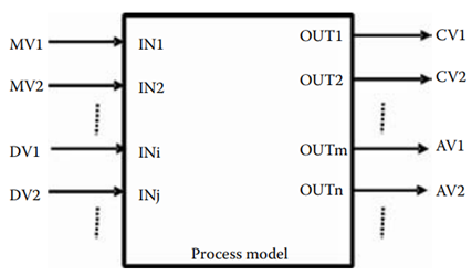
Figure 1.2 [Multivariable MPC-controlled generic process configuration].

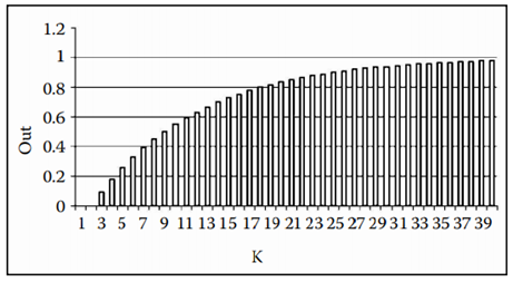
Figure 1.3 [Step response with 40 coefficients].

Manipulated variables, such as process inputs, are subject to hard constraints, meaning that their limits cannot be violated at any time. These constraints can be absolute or incremental in nature. On the other hand, measured disturbances are input variables that are not managed by the MPC controller.

Controlled variables are process outputs that are maintained at specific set points or within predetermined ranges. The prediction horizon, which is the range of process output prediction in scans, is used by process models to predict future values of controlled variables for a certain number of scans.

Constraint variables, a type of controlled variable, are controlled within specified ranges only and do not have set points. These variables are subject to soft constraints, meaning that temporary violations may be allowed to satisfy other system criteria or constraints. Some refer to both controlled variables and constraint variables as controlled variables, differentiating them by using the terms controlled variables with set points and controlled variables with limits, respectively.

The MPC technology relies on the process model as its foundation. Step response models, which provide future predictions of process outputs, are commonly used in most MPC implementations. These models use coefficients that correspond to the step response value at a specific time instance in the future. In other words, the step response is a prediction of the process output for a unit step input applied at scan zero, up to the prediction horizon.

An MPC controller uses an incremental model, where real process input and output values are assigned to the model during initialization. Later on, input increments are considered, and output increments are calculated by the model.

Process Modelling Equations

MPC application assumes a linear process model. Mathematically we can consider a predicted output trajectory of a process as a process state and use a modified state space form for process modelling. For single-input, single-output (SISO) process prediction, the equations are in the form:

(1) $\begin{equation*} \textbf{\textrm{x}}_k = A\textbf{\textrm{x}}_{k-1} + \textbf{\textrm{b}}\Delta u_{k} + \textbf{\textrm{fw}}_{k} \end{equation*}$

(2) $\begin{equation*} \textbf{\textrm{y}}_0 = \textbf{\textrm{Cx}}_{k} \end{equation*}$

where $\textbf{\textrm{x}}_{k-1} = [y_0, y_1, ..., y_i, ..., y_{p-1}]^2$ is the vector of process output prediction at a time $k-1, 0, 1, 2,…, p-1$ steps ahead.

Matrix $\textbf{A}$ is the shift operator defined for a self-regulating process as

$\textbf{A\textrm{x}}_{k-1} = [y_0, y_1, ..., y_i, ..., y_{p-1}]^T$

$\textbf{\textrm{b}} = [b_0, b_1,..., b_i, ..., b_{p-1}]^T$ is the vector of $\textbf{p}$ step response coefficients.

$\textbf{\Delta u_k} = u_k - u_{k-1}$ is the change in process input/controller output.

$w_k = y^p - y^m = y^p - y_0$ is the process output measurement minus the model output (the mismatch between the process and the model that results from the noise, unmeasured disturbances and model inaccuracy).

$\textbf{f}$ is the $p$ dimension filter vector with unity default values.

Matrix $\textbf{C}$ is the operator for selecting the current model output defined as $y_0 = \textbf{\textrm{Cx}}_{k+1}$ .

The MPC controller updates prediction and control calculations every scan. This procedure is known as receding horizon control.

For n outputs and m inputs process, vector $\textbf{\textrm{x}}_k$ has dimension $n ∗ p$ and vector $\textbf{\textrm{b}}$ becomes a matrix $\textbf{\textrm{B}}$ with dimension $n ∗ p$ rows and $m$ columns. The graphical illustration of the equations in Figure 1.4 explains the prediction principles.

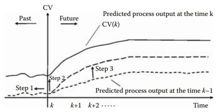
Figure 1.4 [Illustration of linear process modeling. (Copyright 2002, ISA—The Instrumentation, Systems, and Automation Society. All rights reserved. Used with permission of ISA—The Instrumentation, Systems, and Automation Society)].

At any time instance $k$ , the process output prediction (bottom curve) is updated in three steps:

The prediction made at the time $k - 1$ (the bottom dotted curve) is shifted one scan to the left.
The prediction curve is moved to the point to match the current measured process output, for filter coefficient = 1, or in general, prediction shift is $\textbf{\textrm{fw}}_{k}$ .
A step response, scaled by the current change on the process input, is added to the output prediction.

Process Model Identification

MPC is used mainly for multivariable and highly interactive processes. Processes are tested by applying a special pulse test sequence instead of a single step. Then, a process model is built from process test data using mathematics.

Using test data, we can build equations for every output that equal the number of collected samples. The number of collected samples in test data is normally significantly higher than the number of unknown model coefficients. Such equations are solved using the least squares technique. This technique finds coefficients that may not fit perfectly in any equation but fit optimally for all equations, in such a way that the total squared error for all equations is minimal.

The form of the equations used for process modeling is defined by the identification modeling technique. There are a number of identification techniques used. The most common identification techniques are Finite Impulse Response (FIR) and Auto Regressive with eXternal inputs (ARX). FIR identifies pulse response coefficients, as in the following equation for a SISO process:

(3) $\begin{equation*} \Delta y_k = \sum_{i=1}^{p} h_i \Delta u_{k-i} \end{equation*}$

where $p$ is prediction horizon, with a typical default value for MPC model 120; $\Delta y_k$ is change in the process output at the time $k$ ; $\Delta u_{k-i}$ is change in the process input at the time $k-i$ ; and $h_i$ is the pulse response coefficient of the model.

Step response coefficients for the MPC controller are calculated directly from the pulse response as follows:

(4) $\begin{equation*} b_k = \sum_{i=1}^{k} h_i \; \; \; k=1,2, ..., p \end{equation*}$

An advantage of FIR is that it does not require any preliminary knowledge about the process. However, identifying step responses with full prediction horizon with as many as 120 or more coefficients results in low confidence levels of identified coefficient values. Therefore, a shorter horizon with about 60 points is more suitable for a FIR model.

A FIR model with a shorter horizon provides the initial part of the step response that is adequate for defining process dead times using a heuristic approach. On the other hand, the ARX model in the following equation has fewer coefficients, which are defined with higher confidence, provided the process dead times are known.

(5) $\begin{equation*} y_k = \sum_{i=1}^{v} a_i y_{k-i} + \sum_{i=1}^{v} b_i u_{k-d-i} \; \; \; \textrm{for SISO processes.} \end{equation*}$

where $a$ , $v$ are autoregressive and moving average equation orders of ARX; $a = 4$ , $v = 4$ satisfy most applications; $a_i$ , $b_i$ are moving average and autoregressive coefficients of the ARX model; and $d$ is dead time in scans.

Applying FIR first and defining dead times and then applying those dead times for ARX provide the best identification results. Step responses for the MPC controller with any prediction horizon are calculated directly from the previous equation.

For a MIMO process, superposition is applied from all inputs to every output both in FIR and ARX models. An identified model should be validated by applying real input data to the model inputs and comparing the model output with real output. An example of a validation plot is shown in Figure 1.5.

The validation procedure also may include statistical techniques for calculating confidence intervals. Confidence intervals form an area around nominally defined step responses. The true value of the step response coefficients is found within confidence intervals with a predefined confidence (or probability). A 95% confidence interval is normally used.

Model Predictive Controller

Dynamic matrix control (DMC) has historically been the most successful MPC implementation approach, based on a dynamic matrix. A dynamic matrix is used for developing an MPC controller. A dynamic matrix is built from step responses to predict the changes in the process outputs that result from moves of the manipulated variables over the control horizon.

Dynamic matrix $\textbf{\textrm{S}}^u$ as in the following equation, calculates prediction vector $\Delta \textbf{\textrm{x}}_k$ resulting from $\textbf{c}$ future moves of MV, defined by the vector $\Delta \textbf{\textrm{u}}_{(k)}$ .

$\Delta \textbf{\textrm{x}}_{k} = \textbf{\textrm{S}}^u \Delta \textbf{\textrm{u}}_{(k)} = \begin{bmatrix} b_0 & 0 & 0 & . & 0 \\ b_1 & b_0 & 0 & . & 0 \\ b_2 & b_1 & b_0 & . & 0 \\ . & . & . & . & . \\ b_i & b_{i-1} & b_{i-2} & . & b_{i-c+1} \\ . & . & . & . & . \\ b_{p-1} & b_{p-2} & b_{p-3} & . & b_{p-c} \end{bmatrix} \begin{bmatrix} \Delta u_k \\ \Delta u_{k-1} \\ \Delta u_{k-2} \\ . \\ \Delta u_{k+c-1} \end{bmatrix} = \begin{bmatrix} \Delta y_0 \\ \Delta y_1 \\ \Delta y_2 \\ . \\ \Delta y_i \\ . \\ \Delta y_{p-1} \end{bmatrix}$

MPC Formulation

A general formulation of the MPC includes minimization of both the squared sum of predicted control error and the squared sum of calculated controller moves.

To get the desired MPC controller performance, two tuning parameters called penalty on moves and penalty on error are used in the formulation.

The MPC controller objective for minimizing the squared error of the controlled variable includes the penalty on error over the prediction horizon. The objective for minimizing the squared changes in the controller output over the control horizon includes the penalty on moves in the following way:

(6) $\begin{equation*} \min_{\Delta \textrm{MV}(k)} \{|| \Gamma^y [CV(k) - R(k)]||^2 + ||\Gamma^u \Delta \textrm{MV}(k)||^2\} \end{equation*}$

where $CV(k)$ is the controlled output $p$ -step ahead prediction vector; $R(k)$ is the p-step ahead reference trajectory (set point) vector; $\Delta \textrm{MV}(k)$ is the c-step ahead incremental control moves vector; $\Gamma^y$ is a diagonal penalty matrix on the controlled output error; $\Gamma^u$ is a diagonal penalty matrix on the control moves; $p$ is the prediction horizon (number of scans); and $c$ is the control horizon (number of scans).

MPC Equations

The solution for the process with dynamic matrix $\textbf{\textrm{S}}<b>^</b>u$ satisfying Equation 2.17 is in the form:

(7) $\begin{equation*} \Delta \textrm{MV}(k) = (S^{uT} \Gamma^{yT} \Gamma^{y} S^{u} + \Gamma^{uT} \Gamma^{u})^{-1} S^{uT} \Gamma^{yT} \Gamma^{y} E_p (k) \end{equation*}$

where $S^{u}$ is the $p \times c$ process dynamic matrix built from the step responses of dimension $p \times c$ for a SISO model and $pn \times cm$ for a MIMO model with $m$ manipulated inputs and $n$ controlled outputs; and $E_p (k)$ is the error vector over prediction horizon.

The performance of the control algorithm is modified by the adjustable parameters: $p, c, \Gamma^u$ , and $\Gamma^y$ . From an implementation point of view, it is inconvenient to use p and c as tuning parameters. $\Gamma^u$ is a basic controller tuning parameter at the controller generation phase. Increasing $\Gamma^u$ elements makes control less aggressive, and while decreasing $\Gamma^u$ makes the control action more aggressive and the control response faster. It follows from experience that the dead time should be accounted for as a major factor in setting the penalty on moves.

The reference trajectory is applied for online tuning. One trajectory design acts in such a way that instead of penalizing any departure from the trajectory, only those deviations that are below the trajectory or above the set point value are penalized (area A and area C if range = 0, Figure 1.5). In addition, the control error is considered zero if the controlled variable is within range (area C if range > 0).

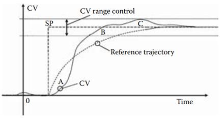
Figure 1.5 [Reference trajectory for funnel control. (Copyright 2002, ISA The Instrumentation, Systems, and Automation Society. All rights reserved. Used with permission of ISA—The Instrumentation, Systems, and Automation Society.)].

Presenting MPC control equation in the form

(8) $\begin{equation*} \Delta \textrm{MV}(k) = \textbf{K}_{mpc} E_{p} (k) \end{equation*}$

where

(9) $\begin{equation*} \textbf{K}_{mpc} = (S^{uT} \Gamma^{yT} \Gamma^{y} S^{u} + \Gamma^{uT} \Gamma^{u})^{-1} S^{uT} \Gamma^{yT} \Gamma^{y}) \end{equation*}$

is the MPC controller gain, one can see that MPC uses integral action. This, however, does not mean that there is a direct analogy between an MPC controller and a conventional, integral-only feedback controller. The major difference is that the MPC controller uses predicted errors and integrates over the prediction horizon.

Integrating MPC, Constraints and Optimisation

A typical MPC configuration includes both controlled variables and constrained variables. The unconstrained MPC controller does not manage constrained variables directly. A supervisory constraint-handling algorithm or optimizer performs the task. The objectives of optimization are usually to maximize a product value and minimize a raw material cost. For processes with an objective function dependent on several manipulated or controlled variables, optimization techniques are essential components of model predictive control technology. The proven optimization technique is linear programming (LP) with steady-state models.

Linear programming is a mathematical technique for solving a set of linear equations and inequalities in order to maximize or minimize an additional function called an objective function. Usually, objective functions express economic value, such as cost or profit.

MPC optimization uses incremental values of MV at the present time or the sum of increments of MV over the control horizon and incremental values of CV at the end of the prediction horizon instead of positional current values, as in typical LP applications. With the prediction horizon normally used in MPC, this assumption guarantees a future steady state for self-regulating processes and perfectly satisfies requirements for proper optimizer operation.

The LP technique uses steady-state models and therefore a steady-state condition is required for its application. The basic steady-state process equation in the incremental form is:

(10) $\begin{equation*} \Delta CV(t + p) = \textbf{\textrm{A}} \Delta \textrm{MV}(t + c) \end{equation*}$

where

(11) $\begin{equation*} \Delta CV(t + p) = \begin{bmatrix} \Delta cv_1 \\ . \\ \Delta cv_n \end{bmatrix} \end{equation*}$

changes in controlled and constraint variables up to the end of prediction horizon.

(12) $\begin{equation*} \textrm{A} = \begin{bmatrix} a_{11} & . & a_{1m} \\ . & . & .\\ a_{n1} & . & a_{nm} \end{bmatrix} \end{equation*}$

process steady-state gain matrix

(13) $\begin{equation*} \Delta \textrm{MV} (t + c) = \begin{bmatrix} \Delta mv_1 \\ . \\ \Delta mv_n \end{bmatrix} \end{equation*}$

changes in manipulating variables to achieve the desired state at the end of control horizon. $\Delta \textrm{MV}$ change should satisfy limits both on $\textrm{MV}$ and $CV$ .

$\textrm{MV}_{MIN} \leq \textrm{MV}_{CURRENT} + \Delta \textrm{MV}_{t+c} \leq \textrm{MV}_{MAX}$

$\textrm{CV}_{MIN} \leq \textrm{CV}_{PREDICTED} + \Delta \textrm{CV}_{t+p} \leq \textrm{CV}_{MAX}$

The objective function for both maximizing output product value and minimizing input raw material cost is defined in the following way:

$Q_{min} = -\textrm{UCV}^T * \Delta \textrm{CV} (t + p) + \textrm{UMV}^T * \Delta \textrm{MV} (t + c)$

where $\textrm{UCV}$ is the cost vector for a $\textrm{CV}$ change of unit value and UMV is the cost vector for an $\textrm{MV}$ change of unit value. Applying equation 1.1, we can express the objective function through $\textrm{MV}$ only:

$Q_{min} = -\textrm{UCV}^T * \textbf{A} * \Delta \textrm{MV} (t + c) + \textrm{UMV}^T * \Delta \textrm{MV} (t + c)$

MPC.01 / Introduction to Multivariable Predictive Control +